Read this article to learn how differentiable programming bridges the gap between classical and quantum machines for the sake of machine learning. The method relies on the fact that the gradient of a quantum circuit can be calculated with regard to the operational parameters. A quantum circuit can function as a node (a QNode) in a traditional neural network if one can calculate its gradients. This page contains more resources on differentiable programming. It’s important to remember that there are numerous ways to implement quantum machine learning. What we present here (and what PennyLane is designed for) has been the leading research concept for a while, but you should be aware that there are different methods out there.
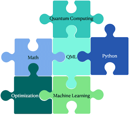
After reading this, you may be asking what steps to take to tackle a problem involving quantum machine learning through programming. Is it possible to use such a program without access to a supercomputer or quantum computer? Thankfully, the correct response is “no.” Several cloud-based quantum computers and portable desktop simulators are at your disposal. Many software libraries exist specifically to facilitate the development and operation of such applications. Figure 1 shows the different technologies are combined and perform according to Quantum Machine Learning.

PennyLane is a Python library that works across platforms and allows for the programmable differentiation of quantum computers. PennyLane facilitates the creation and execution of quantum computing applications through the usage of several suppliers’ quantum machines.
Knowing where your quantum computing program will be executed is essential. A “device” refers to the physical location where your software will be executed. Given the inherent noise in contemporary quantum computers, simulating the problem beforehand is usually the best bet. Since the number of qubits (or wires) in a circuit can vary, it is vital to specify how many qubits your device will have.
Define your QNode once you’ve defined your device; it’ll connect your hardware with a Python function that runs a quantum circuit and produces a value. Parameters can be easily incorporated into circuits using this syntax. Ultimately, a quantum computer is essentially a function that takes in some data and spits out some results.
A cost function can then be defined using the QNode’s output (just like any other normal Python function). Pre- and post-processing in hybrid models can be arbitrarily involved. This allows us to extend its capabilities in a variety of ways, from simply adding a constant to fully integrating a neural network. If you’re set on including a neural network in your cost function, you can accomplish it by first defining the network as a standalone function.
Optimization over the cost function is the last stage. Many different optimizers are available on PennyLane. The optimization process entails picking an optimizer and a step size, making an educated guess about the parameters’ values, and then performing an iterative procedure over a fixed number of steps. When you’re satisfied with your optimization, you may now print or graph the results.
In conclusion, the following steps are required to develop a quantum machine learning application in PennyLane:
- Include the device’s type and wire count in your definition.
- Quantum node (QNode) definition.
- Explain the difference between pre-and post-processing and give an example using a neural network. (Optional)
- Incorporating your quantum circuit and neural network (if present) into a cost function.
- Do the optimum setting to begin, pick an optimizer. Step 2: Determine the size of your increments. Third, hazard a guess at the starting values for your parameters. Repeat a set of predetermined steps over and over.
- Print or graph your findings and take a look.

Author:
Dr. Manish Bhardwaj
Department of Computer Science and Information Technology,
KIET Group of Institutions, Delhi-NCR, Ghaziabad, India
